从零实现一个简单 GNN：邻居之间怎样“传话”

这篇笔记用 PyTorch 手写一个非常小的 GNN/GCN，不依赖 PyTorch Geometric。

你会看到：

1. 图数据和普通表格数据有什么不同。
2. GNN 的核心：每个节点读取邻居的信息，再更新自己。
3. 如何用矩阵乘法实现一次 message passing。
4. 如何把它包装成 nn.Module 并训练一个节点分类模型。

直观比喻：如果每个节点是一个人，边表示谁认识谁，GNN 就像让每个人先听朋友说几句话，再综合自己的信息做判断。

0. 环境准备

导入依赖：

import matplotlib.pyplot as plt
import torch
from torch import nn
import torch.nn.functional as F

torch.manual_seed(7)
print('torch version:', torch.__version__)

1. GNN 能做什么？

GNN 适合处理“对象之间有关系”的数据。常见任务包括：

• 节点分类：社交网络里判断用户兴趣、论文引用网络里判断论文主题。
• 边预测：推荐好友、预测商品和用户是否会交互。
• 整图分类：判断一个分子是否有毒、一个程序调用图是否危险。

今天我们做最小例子：节点分类。

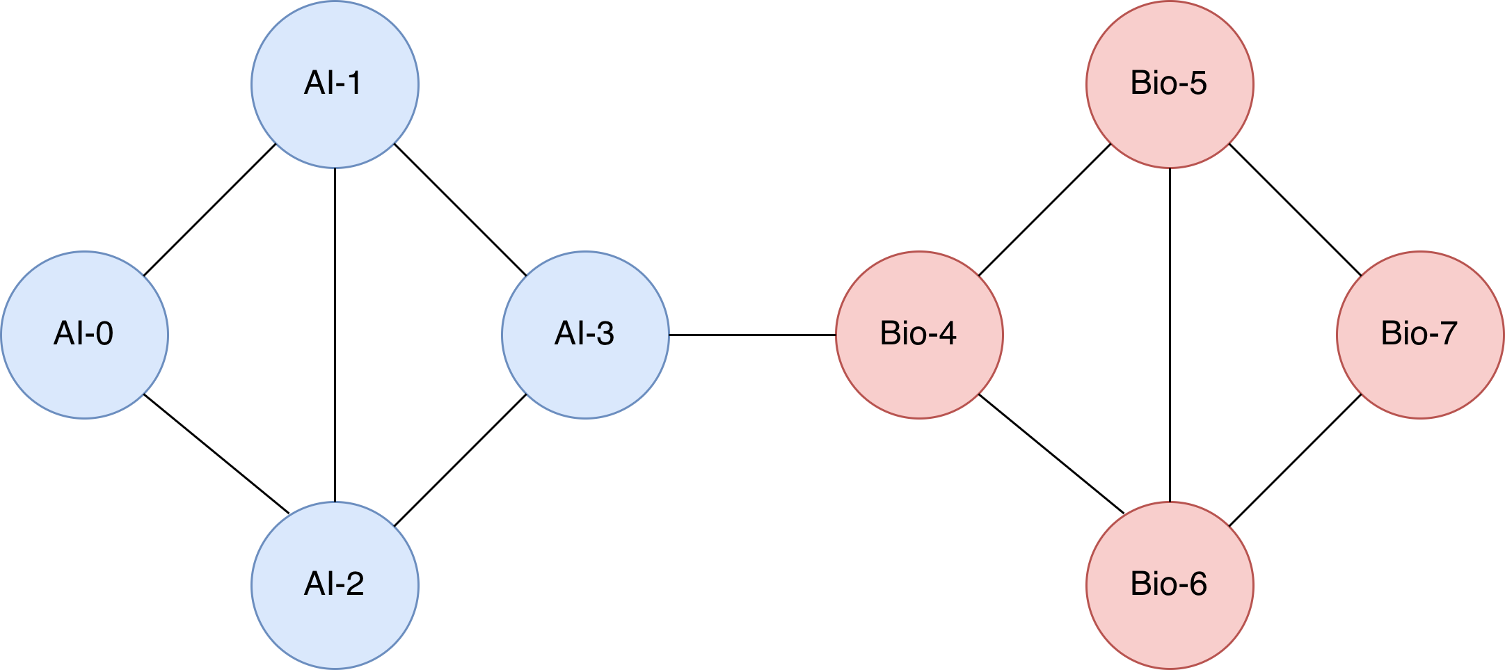
玩具设定：有 8 篇“论文”，它们互相引用。左边一团是 AI 论文，右边一团是生物论文。有些论文自己的关键词很模糊，但它们引用/被引用的邻居能帮我们判断主题。

node_names = [
    'AI-0', 'AI-1', 'AI-2?', 'AI-3?',
    'Bio-4', 'Bio-5', 'Bio-6?', 'Bio-7?',
]

# 标签：0 = AI, 1 = Biology
labels = torch.tensor([0, 0, 0, 0, 1, 1, 1, 1])

# 节点特征：前两个节点有清晰 AI 特征，中间几个是模糊特征。
# 这故意让纯 MLP 很难判断模糊节点，但 GNN 可以借助邻居。
features = torch.tensor([
    [1.0, 0.0, 0.0],  # clear AI
    [1.0, 0.0, 0.0],  # clear AI
    [0.0, 0.0, 1.0],  # ambiguous
    [0.0, 0.0, 1.0],  # ambiguous
    [0.0, 1.0, 0.0],  # clear Biology
    [0.0, 1.0, 0.0],  # clear Biology
    [0.0, 0.0, 1.0],  # ambiguous
    [0.0, 0.0, 1.0],  # ambiguous
])

# 无向边：两个主题各自内部连接紧密，节点 3 和 4 之间有一条弱桥。
edges = [
    (0, 1), (0, 2), (1, 2), (1, 3), (2, 3),
    (4, 5), (4, 6), (5, 6), (5, 7), (6, 7),
    (3, 4),
]

num_nodes = len(node_names)
adjacency = torch.zeros(num_nodes, num_nodes)
for i, j in edges:
    adjacency[i, j] = 1
    adjacency[j, i] = 1

print('features shape:', tuple(features.shape))
print('adjacency shape:', tuple(adjacency.shape))
adjacency

示例输出：

features shape: (8, 3)
adjacency shape: (8, 8)

tensor([[0., 1., 1., 0., 0., 0., 0., 0.],
        [1., 0., 1., 1., 0., 0., 0., 0.],
        [1., 1., 0., 1., 0., 0., 0., 0.],
        [0., 1., 1., 0., 1., 0., 0., 0.],
        [0., 0., 0., 1., 0., 1., 1., 0.],
        [0., 0., 0., 0., 1., 0., 1., 1.],
        [0., 0., 0., 0., 1., 1., 0., 1.],
        [0., 0., 0., 0., 0., 1., 1., 0.]])

邻接矩阵是一个 8 x 8 矩阵。第 i 行第 j 列为 1 表示节点 i 和节点 j 有边相连；为 0 表示没有直接连接。图结构如下图所示：

2. 一次 message passing 等于什么？

最朴素的想法：每个节点把邻居特征取平均。

但节点也应该保留自己的信息，所以先给图加 self-loop：每个节点连向自己。

公式上，一次邻居平均可以写成：

其中：

• 是邻接矩阵。
• 是 self-loop。
• 是度矩阵，用来做平均。
• 是节点特征。

adjacency_with_self = adjacency + torch.eye(num_nodes)
degree = adjacency_with_self.sum(dim=1, keepdim=True)
mean_aggregator = adjacency_with_self / degree

mixed_features = mean_aggregator @ features

print('原始特征 X:')
print(features)
print('\n经过一次邻居平均后的特征 D^-1(A+I)X:')
print(mixed_features.round(decimals=2))

示例输出：

原始特征 X:
tensor([[1., 0., 0.],
        [1., 0., 0.],
        [0., 0., 1.],
        [0., 0., 1.],
        [0., 1., 0.],
        [0., 1., 0.],
        [0., 0., 1.],
        [0., 0., 1.]])

经过一次邻居平均后的特征 D^-1(A+I)X:
tensor([[0.6700, 0.0000, 0.3300],
        [0.5000, 0.0000, 0.5000],
        [0.5000, 0.0000, 0.5000],
        [0.2500, 0.2500, 0.5000],
        [0.0000, 0.5000, 0.5000],
        [0.0000, 0.5000, 0.5000],
        [0.0000, 0.5000, 0.5000],
        [0.0000, 0.3300, 0.6700]])

观察上面的输出：模糊节点 [0, 0, 1] 在和 AI 邻居混合后，会带上 AI 分量；和 Biology 邻居混合后，会带上 Biology 分量。

这就是 GNN 的核心价值：节点不只看自己，还看自己处在什么关系网络里。

3. GCN 层：邻居聚合 + 可学习变换

真正的神经网络需要可学习参数。经典 GCN 的一层可写成：

为了训练更稳定，常用对称归一化：

def normalize_adjacency(adjacency_matrix):
    adjacency_with_self = adjacency_matrix + torch.eye(adjacency_matrix.size(0))
    degree = adjacency_with_self.sum(dim=1)
    degree_inv_sqrt = torch.pow(degree, -0.5)
    degree_inv_sqrt[torch.isinf(degree_inv_sqrt)] = 0.0
    d_inv_sqrt = torch.diag(degree_inv_sqrt)
    return d_inv_sqrt @ adjacency_with_self @ d_inv_sqrt

adjacency_norm = normalize_adjacency(adjacency)
adjacency_norm.round(decimals=2)

运行，输出对称归一化后的邻接矩阵如下：

tensor([[0.3300, 0.2900, 0.2900, 0.0000, 0.0000, 0.0000, 0.0000, 0.0000],
        [0.2900, 0.2500, 0.2500, 0.2500, 0.0000, 0.0000, 0.0000, 0.0000],
        [0.2900, 0.2500, 0.2500, 0.2500, 0.0000, 0.0000, 0.0000, 0.0000],
        [0.0000, 0.2500, 0.2500, 0.2500, 0.2500, 0.0000, 0.0000, 0.0000],
        [0.0000, 0.0000, 0.0000, 0.2500, 0.2500, 0.2500, 0.2500, 0.0000],
        [0.0000, 0.0000, 0.0000, 0.0000, 0.2500, 0.2500, 0.2500, 0.2900],
        [0.0000, 0.0000, 0.0000, 0.0000, 0.2500, 0.2500, 0.2500, 0.2900],
        [0.0000, 0.0000, 0.0000, 0.0000, 0.0000, 0.2900, 0.2900, 0.3300]])

定义图卷积层和图卷积神经网络模型如下：

class GraphConvolution(nn.Module):
    """A minimal GCN layer: output = A_norm @ Linear(node_features)."""

    def __init__(self, in_features, out_features):
        super().__init__()
        self.linear = nn.Linear(in_features, out_features, bias=False)

    def forward(self, node_features, adjacency_norm):
        transformed = self.linear(node_features)
        return adjacency_norm @ transformed


class TinyGCN(nn.Module):
    def __init__(self, in_features, hidden_features, num_classes):
        super().__init__()
        self.gcn1 = GraphConvolution(in_features, hidden_features)
        self.gcn2 = GraphConvolution(hidden_features, num_classes)

    def forward(self, node_features, adjacency_norm):
        hidden = self.gcn1(node_features, adjacency_norm)
        hidden = F.relu(hidden)
        logits = self.gcn2(hidden, adjacency_norm)
        return logits


model = TinyGCN(in_features=3, hidden_features=8, num_classes=2)
print(model)

这里有两个关键点：

• Linear 负责学习如何变换节点特征。
• adjacency_norm @ transformed 负责把邻居信息传播过来。

4. 训练：只给少数节点标签

我们只把 0、1、4、5 这四个“特征清晰”的节点作为训练集。

模型要把图结构中的信息传播到 2、3、6、7 这些模糊节点上。

train_mask = torch.tensor([True, True, False, False, True, True, False, False])
test_mask = ~train_mask

optimizer = torch.optim.Adam(model.parameters(), lr=0.05, weight_decay=1e-3)

history = []
for epoch in range(25):
    model.train()
    optimizer.zero_grad()

    logits = model(features, adjacency_norm)
    loss = F.cross_entropy(logits[train_mask], labels[train_mask])

    loss.backward()
    optimizer.step()

    with torch.no_grad():
        prediction = logits.argmax(dim=1)
        train_acc = (prediction[train_mask] == labels[train_mask]).float().mean().item()
        test_acc = (prediction[test_mask] == labels[test_mask]).float().mean().item()
        history.append((loss.item(), train_acc, test_acc))

    if (epoch+1) % 5 == 0:
        print(f'epoch={epoch+!:03d} loss={loss.item():.4f} train_acc={train_acc:.2f} test_acc={test_acc:.2f}')

示例输出：

epoch=005 loss=0.5736 train_acc=0.75 test_acc=0.50
epoch=010 loss=0.3862 train_acc=1.00 test_acc=0.75
epoch=015 loss=0.1861 train_acc=1.00 test_acc=0.75
epoch=020 loss=0.0558 train_acc=1.00 test_acc=1.00
epoch=025 loss=0.0124 train_acc=1.00 test_acc=1.00

绘制训练曲线：

losses, train_accs, test_accs = zip(*history)
plt.figure(figsize=(8, 3))
plt.subplot(1, 2, 1)
plt.plot(losses)
plt.title('Training loss')
plt.xlabel('epoch')

plt.subplot(1, 2, 2)
plt.plot(train_accs, label='train')
plt.plot(test_accs, label='test')
plt.ylim(-0.05, 1.05)
plt.title('Accuracy')
plt.xlabel('epoch')
plt.legend()
plt.tight_layout()
plt.show()

查看每个节点的预测结果：

model.eval()
with torch.no_grad():
    logits = model(features, adjacency_norm)
    probabilities = logits.softmax(dim=1)
    predictions = logits.argmax(dim=1)

for i, name in enumerate(node_names):
    true_label = 'AI' if labels[i].item() == 0 else 'Bio'
    pred_label = 'AI' if predictions[i].item() == 0 else 'Bio'
    split = 'train' if train_mask[i] else 'test '
    confidence = probabilities[i, predictions[i]].item()
    print(f'{name:6s} [{split}] true={true_label:3s} pred={pred_label:3s} confidence={confidence:.2f}')

示例输出：

AI-0   [train] true=AI  pred=AI  confidence=0.99
AI-1   [train] true=AI  pred=AI  confidence=0.98
AI-2?  [test ] true=AI  pred=AI  confidence=0.98
AI-3?  [test ] true=AI  pred=AI  confidence=0.77
Bio-4  [train] true=Bio pred=Bio confidence=0.99
Bio-5  [train] true=Bio pred=Bio confidence=1.00
Bio-6? [test ] true=Bio pred=Bio confidence=1.00
Bio-7? [test ] true=Bio pred=Bio confidence=0.99

5. 小结

GNN 的基本套路可以压缩成三句话：

1. 每个节点有自己的特征，图告诉我们节点之间有什么关系。
2. 一层 GNN 让节点聚合邻居信息，再用可学习参数变换。
3. 多层 GNN 就是在更大范围内传递信息：一层看一跳邻居，两层看两跳邻居。

这个例子只实现了最小 GCN。真实项目会继续考虑大图采样、稀疏矩阵、边特征、动态图、过平滑、归纳泛化等问题。